Standard Process
- Feature engineering
- Split the data into train and test sets (random or not)
- Based on the train data set, apply cross validation to choose optimal tuning parameter for regularized models, like lasso, ridge and elastic net.
- Based on entire training data set, fit all regularized models with best tuning parameter and fit the base linear model as well.
- Apply the test data set to select the best model.
- Check more statistics.
- Check specific features and go back to adjust model.
Prepreparation in python 3
1. Import some necessary packages
import pandas as pd
from pandas import DataFrame
import numpy as np
import matplotlib.pyplot as plt
import seaborn as sns
from sklearn.datasets import load_diabetes
from sklearn.linear_model import Lasso, Ridge, ElasticNet, LinearRegression
from sklearn.cross_validation import cross_val_score, train_test_split, KFold
from sklearn.grid_search import GridSearchCV
from sklearn.metrics import r2_score, mean_squared_error
import statsmodels.api as sm
2. Toy data set
diabetes = load_diabetes()
This data set has 10 features diabetes.data and one target diabetes.target. Besides, there is no description of this data set, so we need to do some feature engineering first.
Feature Engineering
Remember that the first thing for feature engineering is to imagine you are the expert in that specific area that your data comes from. From expert perspective, you can select features based on professional experience (just google it as much as you can).
1. Check whether this data set is normalized
X = diabetes['data']
X = DataFrame(X)
X.describe()
We can tell from this description of each feature that the mean value is around 0 and has same standard deviation. Therefore, the predictors are normalized.
In other datasets, the X may not be centered, then we need to add the intercept. In sklearn, there is one argument to add intercept fit_intercept = True. The alternative way is:
sm.add_constant(X)
2. Check the correlation of features and target
diabetes_df = DataFrame(diabetes.data)
diabetes_df.columns = ["X" + str(col) for col in diabetes_df.columns]
diabetes_df["target"] = diabetes.target
3. Plot the scatter points of each feature against target
From the pair plot figure we can tell the relationship of features and target and the relationship between features. There may be some features do not have linear relationship with target, we can try to guess any function in our knowledge have the similar curves with those nonlinear relationship. If we detect some strong correlated features, we should be really careful. When two features are linearly correlated, we need to remove one of them from analysis. When two features have nonlinear relationship, we still need to guess the function that can describe this relationship best.
sns.pairplot(diabetes_df)
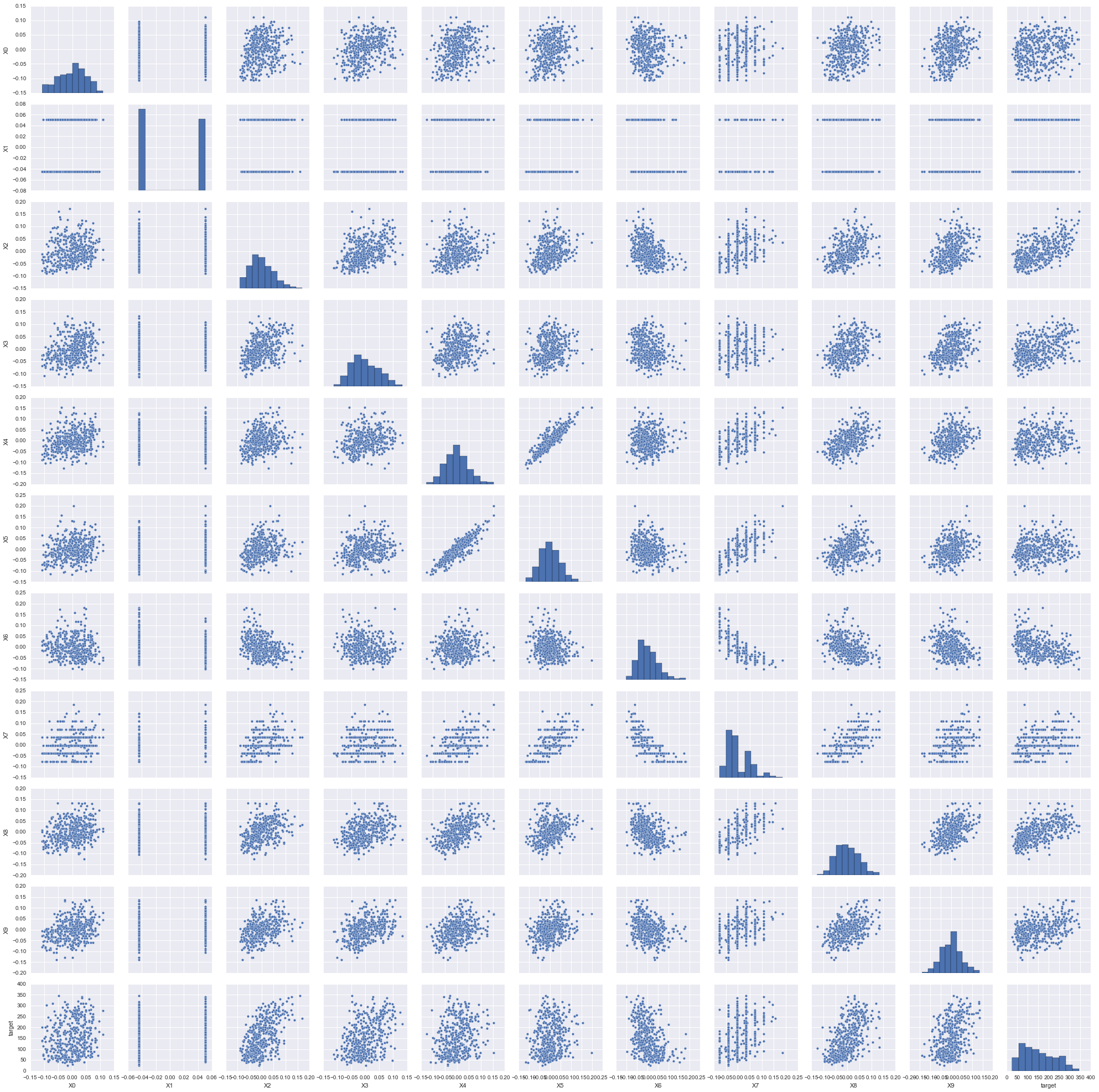
We can tell from this pair plot figure that there are two categorical features and it is not necessary to apply polynomial regression.
Split the data
Since we need to compare the results from multiple models, we need to split the data into train and test sets.
X_train, X_holdout, y_train, y_holdout = train_test_split(diabetes.data, diabetes.target, test_size=0.1, random_state=42)
In this case, we need to shuffle the data before we split data. However in some other cases, we need to apply different strategies. If the data is in time series, then we may not need to shuffle the data. If target is categorical, then we need to use stratified k-fold.
Cross Validation
Now we need to apply cross validation to choose tuning parameter in regularized models.
1. Split train data into multiple folds
kfold = KFold(len(X_train), n_folds=5, shuffle=True, random_state=0)
In this case, we need to shuffle the data before we split data (even if the data is in time series). If target is categorical, then we need to use stratified k-fold.
from sklearn.cross_validation import StratifiedKFold
X = np.array([[1, 2], [3, 4], [1, 2], [3, 4]])
y = np.array([0, 0, 1, 1])
skf = StratifiedKFold(y, n_folds=2)
for train_index, test_index in skf:
   print("TRAIN:", train_index, "TEST:", test_index)
   X_train, X_test = X[train_index], X[test_index]
   y_train, y_test = y[train_index], y[test_index]
   #Then fit and test your model.
TRAIN: [1 3] TEST: [0 2]
TRAIN: [0 2] TEST: [1 3]
2. Select best tuning parameter
Apply grid search and cross validation to find the optimal tuning parameters in the lasso, ridge and elastic net models. Compared with lasso penalty, ridge (L2) penalizes less on small numbers and more on large numbers. Elastic net tries to balance these two penalties.
def cv_optimize(clf, parameters, X, y, n_folds, n_jobs=1, score_func=None):
    if score_func:
        gs = GridSearchCV(clf, param_grid=parameters, cv=n_folds, n_jobs=n_jobs, scoring=score_func)
    else:
        gs = GridSearchCV(clf, param_grid=parameters, n_jobs=n_jobs, cv=n_folds)
    gs.fit(X, y)
    print ("BEST", gs.best_params_, gs.best_score_)
    df = pd.DataFrame(gs.grid_scores_)
    #Plot mean score vs. alpha
    for param in parameters.keys():
        df[param] = df.parameters.apply(lambda val: val[param])
    plt.semilogx(df.alpha, df.mean_validation_score)
    return gs
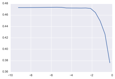
1) Lasso
params = {
    "alpha": np.logspace(-4, -.1, 20)
}
#If we do not know whether we need to normalize the data first, we can do this:
#params = {
#    "alpha": np.logspace(-4, -.1, 20), "normalize": [False, True]
#}
lm_lasso = cv_optimize(Lasso(), params, X_train, y_train, kfold)
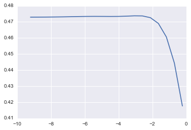
2) Ridge
params = {
    "alpha": np.logspace(-4, -.1, 20)
}
lm_ridge = cv_optimize(Ridge(), params, X_train, y_train, kfold)
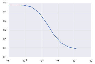
3)Elastic Net
params = {
    "alpha": np.logspace(-4, -.1, 20)
}
lm_elastic = cv_optimize(ElasticNet(), params, X_train, y_train, kfold)
Fit models with best parameters
Now we will fit the linear regression models with or without penalties.
lm_lasso_best = Lasso(alpha = lm_lasso.best_params_['alpha']).fit(X_train, y_train)
lm_ridge_best = Lasso(alpha = lm_ridge.best_params_['alpha']).fit(X_train, y_train)
lm_elasticnet_best = Lasso(alpha = lm_elasticnet.best_params_['alpha']).fit(X_train, y_train)
lm_base = LinearRegression().fit(X_train, y_train)
y_lasso = lm_lasso_best.predict(x_holdout)
y_ridge = lm_ridge_best.predict(x_holdout)
y_elasticnet = lm_elasticnet_best.predict(x_holdout)
y_base = lm_base.predict(x_holdout)
mse_lasso = np.mean((y_lasso - y_holdout) ** 2)
mse_ridge = np.mean((y_ridge - y_holdout) ** 2)
mse_elasticnet = np.mean((y_elasticnet - y_holdout) ** 2)
mse_base = np.mean((y_base - y_holdout) ** 2)

print("Linear Regression: R squred score is ", r2_score(y_holdout, y_base), " and mean squred error is ", mse_base)
print("Lasso Regression: R squred score is ", r2_score(y_holdout, y_lasso), " and mean squred error is ", mse_lasso)
print("Ridge Regression: R squred score is ", r2_score(y_holdout, y_ridge), " and mean squred error is ", mse_ridge)
print("Elastic Net Regression: R squred score is ", r2_score(y_holdout, y_elasticnet), " and mean squred error is ", mse_elasticnet)
Then we can choose the best models with best R squred score and mean squared errors.
More statistics
In many situations, we want to check more statistics of linear regression. We can apply t statistic to select features with base linear regression. The smaller p-value of t statistic means more significance of that feature. Typically when p-value is larger than 0.05 we say that feature is not important. To do this, we need to use package statsmodels.api.
#X_train = sm.add_constant(X_train)      #if data is not centered.
model = sm.OLS(y_train, X_train)
results = model.fit()
results.summary()
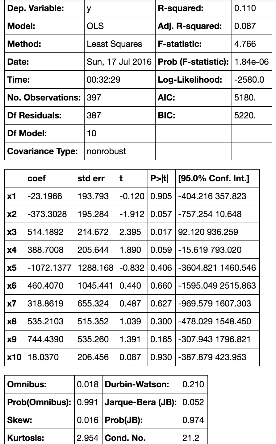
This table can provide a lot of statistical analysis information. From this table, if we set significance level as 0.05 there are only two significant features. However we still cannot simply decide to get rid of those unimportant features.
Check specific features
If some features are ruled out by regularization regression or have very large p-value, we need to plot the points and fitted line to make a double check. It may be caused by noisy features, non-linear relationship or correlated features.
Xt = X_train[:,2]    #Check third feature.
X_line = np.linspace(min(Xt),max(Xt), 10).reshape(10,1)
X_line = np.tile(X_line, [1, 10])
y_train_pred = lin_reg_est.predict(X_line)
plt.scatter(Xt, y_train, alpha=0.2)
plt.plot(X_line, y_train_pred)
plt.show()
Some further discussion about normalization (centering and scaling):
- centering is equivalent to adding the intercept
- when you’re trying to sum or average variables that are on different scales, perhaps to create a composite score of some kind. Without scaling, it may be the case that one variable has a larger impact on the sum due purely to its scale, which may be undesirable.
- To simplify calculations and notation. For example, the sample covariance matrix of a matrix of values centered by their sample means is simply \(X′X\). Similarly, if a univariate random variable \(X\) has been mean centered, then \(var(X)=E(X^2)\) and the variance can be estimated from a sample by looking at the sample mean of the squares of the observed values.
- PCA can only be interpreted as the singular value decomposition of a data matrix when the columns have first been centered by their means.
Note that scaling is not necessary in the last two bullet points I mentioned and centering may not be necessary in the second bullet I mentioned, so the two do not need to go hand and hand at all times. For regression without regularization centering and scaling are not necessary, but centering is helpful for interpretation of coefficients. For regularized regression, centering (or adding intercept) is necessary because we want coefficients have same magnitude.
Remarks and Tips
- If the data size is very large, then grid search and cross validation will cost too much time. Therefore we may use small number of folds and small candidate sets of parameters.
- Before split data and fit model you need to make sure that your features are in columns. Especially when you have only one feature, you may apply
np.reshape(). - If the data set was not centered, we need to set the
intercept = Trueinside each model. - sklearn and statsmodels.api apply different algorithm to fit the linear model, so they will out put different results.
- Another way to use regularization models is to apply them select features, then use base linear regression to analyze data with selected features